Multi-Label Facial Attribute Classification with CNN
This project builds a deep learning model to predict multiple visual attributes from a single face image. Unlike standard image classification, each image can have many labels at once, such as hair color, facial expression, accessories, and other visible attributes. The final workflow compares a baseline neural network, a tuned MLP, and a convolutional neural network before improving the decision threshold strategy for multi-label prediction.
The notebook was originally developed in Kaggle and has been adapted to run locally with TensorFlow/Keras. The local version reads the CelebA metadata and image files from the project folder, loads saved .keras models, and supports repeatable evaluation from the saved CNN model.
The full implementation is available in CNN_Celeb.ipynb, with local setup notes in README.md.
Project Objective
The goal was to develop a model that can predict 40 facial attributes per image and evaluate it using metrics that are appropriate for imbalanced multi-label classification.
Rather than focusing only on binary accuracy, the analysis uses Micro-F1, Macro-F1, Hamming Loss, and mean average precision. This is important because the CelebA attributes are not evenly distributed: common labels can make overall accuracy look strong, while rarer labels may still be missed.
Dataset and Task Design
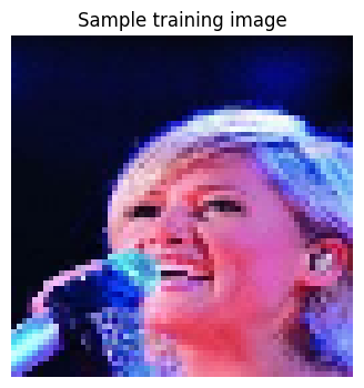
The project uses the CelebA aligned face image dataset with 40 binary attributes. The original labels are encoded as 1 and -1, then converted to 1 and 0 for multi-label training.
Dataset
CelebA aligned face images with official train, validation, and test partitions.
Target
40 independent facial attribute labels predicted for each image.
Input Shape
Images resized to 64 x 64 x 3, normalized to the range 0 to 1.
The preprocessing pipeline uses tf.data to read image paths, decode JPEG files, resize images, normalize pixel values, batch samples, and prefetch data for training. This keeps the image loading workflow scalable while preserving the official train/validation/test split.
Modeling Approach
The project was structured as three stages so that the CNN result could be interpreted against simpler baselines.
| Stage | Model | Purpose |
|---|---|---|
| Q1 | Baseline MLP | Establish a simple benchmark using flattened image pixels. |
| Q2 | Tuned MLP | Test whether additional dense capacity, dropout, batch normalization, learning rate scheduling, and regularization improve performance. |
| Q3 | CNN | Use convolutional layers to capture spatial image patterns before multi-label prediction. |
The final CNN uses three convolutional blocks with filter sizes 32, 64, and 128. Each block applies a 3 x 3 convolution with same padding and ReLU activation, followed by max pooling. The extracted spatial features are flattened and passed through a dense layer before a 40-unit sigmoid output layer.
Input image: 64 x 64 x 3
Data augmentation: random flip, rotation, zoom
Conv2D 32 + MaxPooling
Conv2D 64 + MaxPooling
Conv2D 128 + MaxPooling
Flatten
Dense 128 + Dropout
Dense 40 sigmoid outputs
The model was trained with binary cross-entropy because each label is treated as an independent binary target. AdamW was used for optimization, with early stopping on validation loss to reduce overfitting.
Performance Improvement Actions
Model performance was improved through a combination of architecture changes, data augmentation, regularization, optimizer tuning, and threshold selection. This was important because the task is both image-based and imbalanced: the model needs to learn visual patterns while also avoiding a bias toward only the most common attributes.
| Improvement Area | Action Taken | Why It Helped |
|---|---|---|
| Spatial feature learning | Replaced flattened-pixel MLPs with a CNN. | Convolutional filters preserve local visual structure such as hair regions, facial contours, and accessory patterns. |
| Geometric augmentation | Applied random horizontal flip, small rotation, and zoom during training. | Exposes the model to realistic image variation so it does not overfit to a single face alignment or crop position. |
| Regularization | Added dropout after the dense layer. | Reduces reliance on a small set of high-activation features and improves generalization. |
| Optimizer tuning | Used AdamW with weight decay. | Combines adaptive learning with mild weight regularization. |
| Early stopping | Monitored validation loss with patience of 2. | Stops training once validation performance stops improving, reducing over-training. |
| Threshold tuning | Compared default 0.50, global tuned threshold, and per-attribute thresholds. |
Improves Macro-F1 by adapting decisions to different label frequencies and probability distributions. |
The augmentation step is especially relevant for the CNN. The implemented notebook uses RandomFlip("horizontal"), RandomRotation(0.03), and RandomZoom(0.05). These transformations create slightly different versions of the same training images, helping the model become less sensitive to small changes in pose, framing, and alignment. A skew or shear transform would follow the same idea if added later: it would simulate mild perspective or face-position variation so the model learns more robust visual features rather than memorizing the exact training image geometry.
The experiments also showed that more complexity was not always better. Deeper CNN variants, larger dense layers, batch normalization, and heavier dropout did not consistently improve Macro-F1. The final model therefore kept the CNN compact and used light augmentation plus mild regularization instead of making the architecture unnecessarily large.
Experiment Findings
The baseline MLP reached reasonable binary accuracy, but its Macro-F1 was much lower than its Micro-F1. This showed that the model was doing better on common attributes than on less frequent ones.
The tuned MLP improved over the first baseline, especially when the dense layers were widened. However, additional depth, batch normalization, learning rate scheduling, and regularization did not produce large gains. This suggested that the MLP was limited by the loss of spatial structure after flattening the image.
The CNN improved the Macro-F1 score by learning local image features directly from the image grid. Data augmentation provided additional robustness, while early stopping helped keep validation and test performance close.
| Model | Test Binary Accuracy | Test Hamming Loss | Test Micro-F1 | Test Macro-F1 | Test Micro-mAP | Test Macro-mAP |
|---|---|---|---|---|---|---|
| Baseline MLP | 0.88 | 0.11 | 0.72 | 0.54 | 0.84 | 0.65 |
| Tuned MLP | 0.8899 | 0.1101 | 0.7424 | 0.5999 | 0.8565 | 0.6824 |
| CNN at 0.50 threshold | 0.8975 | 0.1025 | 0.7620 | 0.6183 | 0.8750 | 0.7225 |
Training and Validation Diagnostics
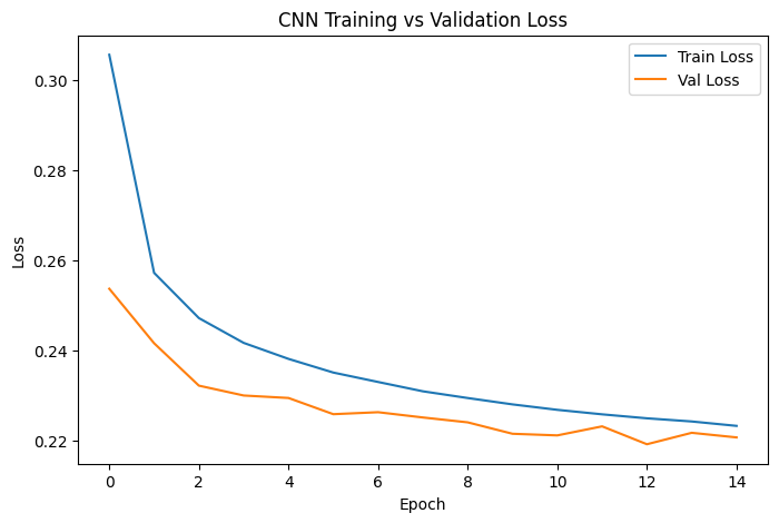
The CNN training curves show how the final model behaved during fitting. Training and validation loss both decreased quickly in the early epochs, then began to flatten. This supports the use of early stopping because additional epochs would provide limited improvement and could increase the risk of overfitting.
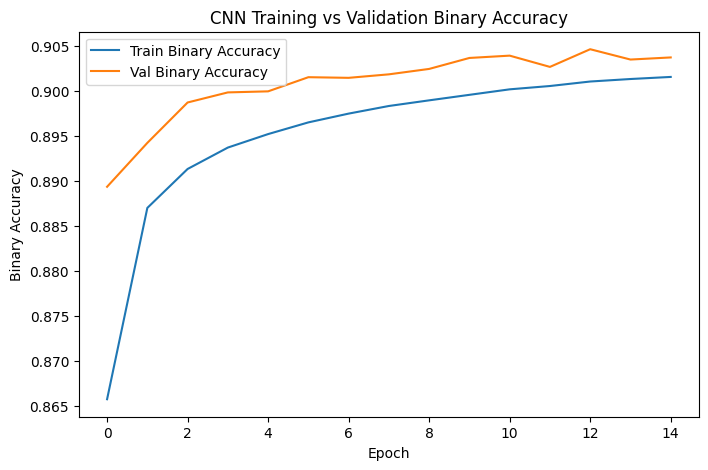
The binary accuracy curve shows a similar pattern. Training accuracy and validation accuracy increased together and stayed close, which suggests that the CNN learned useful image features without a large generalization gap.
At the default 0.50 threshold, validation and test performance were also close. This gave confidence that the CNN was not only fitting the validation set, but was transferring reasonably well to unseen test images.
| Dataset | Binary Accuracy | Hamming Loss | Micro-F1 | Macro-F1 | Micro-mAP | Macro-mAP |
|---|---|---|---|---|---|---|
| Validation | 0.9047 | 0.0953 | 0.7720 | 0.6274 | 0.8775 | 0.7253 |
| Test | 0.8975 | 0.1025 | 0.7620 | 0.6183 | 0.8750 | 0.7225 |
Threshold Optimization
A fixed threshold of 0.50 is often too rigid for multi-label classification. Different attributes have different prevalence rates and probability distributions, so a single threshold can create too many false negatives for rarer attributes.
Two threshold strategies were evaluated:
| Threshold Strategy | Test Binary Accuracy | Test Hamming Loss | Test Micro-F1 | Test Macro-F1 | Test Micro-mAP | Test Macro-mAP |
|---|---|---|---|---|---|---|
Global threshold tuned on validation set: 0.30 |
0.8804 | 0.1196 | 0.7635 | 0.6709 | 0.8750 | 0.7225 |
| Per-attribute thresholds tuned on validation set | 0.8838 | 0.1162 | 0.7638 | 0.6825 | 0.8750 | 0.7225 |
The per-attribute threshold strategy produced the best Macro-F1 score. This means it improved balance across the 40 attributes, even though binary accuracy decreased slightly compared with the default 0.50 threshold.
Mean average precision stayed unchanged because mAP is calculated from the predicted probabilities before thresholding. This makes mAP useful for judging ranking quality, while F1-based metrics show how well the chosen threshold converts probabilities into final labels.
Final Result
The final selected result is the CNN with per-attribute threshold tuning.
| Metric | Result | Interpretation |
|---|---|---|
| Binary Accuracy | 0.8838 | Correct label decisions across all image-label pairs. |
| Hamming Loss | 0.1162 | About 11.6% of label assignments were incorrect. |
| Micro-F1 | 0.7638 | Strong overall label-instance performance, influenced by common labels. |
| Macro-F1 | 0.6825 | Better balance across common and rare attributes after threshold tuning. |
| Micro-mAP | 0.8750 | Strong probability ranking across all label instances. |
| Macro-mAP | 0.7225 | More challenging, but reasonable, ranking performance across labels. |
Key Learnings
This project showed that CNNs are more suitable than flattened-pixel MLPs for image-based multi-label prediction because convolutional filters preserve local spatial patterns. It also showed that threshold selection is not a small post-processing detail: for imbalanced multi-label problems, threshold tuning can materially improve Macro-F1 and make the model fairer across labels.
The most important modeling lesson was that the best model was not the largest architecture. A compact CNN with light augmentation, mild dropout, AdamW optimization, and early stopping generalized better than deeper or heavily regularized alternatives.
Future Improvements
- Add per-label precision, recall, and F1 tables to identify the strongest and weakest attributes.
- Display example image predictions with true labels, predicted labels, and confidence scores.
- Explore transfer learning with pretrained image backbones such as MobileNetV2 or EfficientNet.
- Test class weighting or focal loss for rare attributes.
- Calibrate probabilities before threshold tuning to improve confidence interpretability.